Vector Spaces

Picture a vector space: large and expansive with no ends in sight. Subtle tick-marks line the ether. There are an arbitrary number of dimensions; any finite number n will do (infinite-dimensional vector spaces make up a different field of study).

Picture a basis in this vector space: a set of vectors which demarcate the space. Points in the vector space are described through their coordinates with respect to a particular basis. Linear algebra vastly generalizes the coordinate system: the “axes” (basis vectors) may be arbitrary in number (as the space is arbitrary in dimension) and they need not be perpendicular nor of equal lengths. These basis vectors simply must be (a) linearly independent (or non-redundant) and (b) span the whole space. Any single vector on a line, or two non-colinear vectors on a plane, or three non-coplanar vectors in three-space, are linearly independent – they can’t be expressed as combinations of each other – and they are a spanning set – the whole space can be accessed through their combinations. Dimension, as it turns out, describes nothing more than the maximum possible number of linearly independent vectors – how many unique vectors might one introduce? or, equivalently, the minimum number of spanning vectors – how many must we add to span the whole space? Such a “minimum spanning set” is called a basis. Can you imagine a fourth vector that can’t be described through some sum the other three, or a space which requires four vectors to span? Then you have imagined the fourth dimension.

Picture a linear transformation: a function, or mapping, which takes each vector in the space and maps it to another vector. A mapping might project each vector in R³ onto the xy-plane; a mapping might rotate the entire space about an axis; a mapping might re-assign vectors wildly. These mappings, or “linear transformations”, operate by producing a new basis from the old; they assign, to each old basis vector e, a new basis vector f expressed uniquely in terms of a set of coordinates a with respect to the old basis vectors. These new coordinates – n² of them (n old-vector coordinates for each of the n new vectors) – are the bits of information required to fully describe our linear transformation. We assemble them in a matrix which uniquely represents the transformation.

Picture, somewhere in this twisting space, a single vector which does not jump wildly but, through some coalescence, simply changes its length. For these vectors, called eigenvectors, the transformation simply multiplies the vector by a scalar, changing its length by eigenvalue λ. In other words, each coordinate c becomes λc. How might we find these vectors? Using the rows of the matrix to describe the transformation of the coordinates, we seek a vector satisfying the relationship on the left; a quick subtraction yields the system on the right.

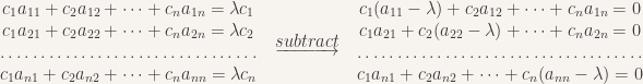
Now, things leap into the world of the strange and unknown. In linear algebra, there’s a special function called the determinant which has many special properties. For one, the determinant can be used to tell us whether, for a system of equations, there exists a solution which is non-trivial, i.e. there are coordinates satisfying the above right-side equation such that all the c’s are not equal to zero (if they were all zero, the system would be trivially satisfied). If the determinant equals zero, there exist non-trivial solutions. In other words, if we apply the determinant to the system of a‘s on the right, set it equal to zero, and solve for lambda, we will produce the lambdas which allow for non-trivial eigenvectors. We get a long polynomial, called the “characteristic polynomial”, over lambda:

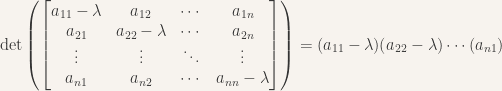
THE ROOTS OF THE CHARACTERISTIC POLYNOMIAL PRODUCE THE TRANSFORMATION’S EIGENVALUES. In other words, we’ve somehow moved from a rigid vector space of lines and dimensions to a flowing, curving polynomial of one variable, whose zeros signal special vectors in our linear transformation. How did we move from one world to the other? I will end with some extra “bonuses” – these might require some further thought for the marvelous insanity to sink in.

1. The characteristic polynomial of a particular linear transformation is independent of the choice of basis.
2. Because a odd-degree polynomial over the real numbers must have at least one root, any linear transformation over odd-dimensional space must have at least one eigenvector.
   
3. If the inner product (or dot product) of two vectors x and y is denoted by (x, y), then for every linear transformation A there exists a unique adjoint transformation A* such that (Ax, y) = (x, A*y). What is the relationship, algebraically as well as geometrically, between a linear transformation and its adjoint?
   
4. In the study of vector spaces over the complex numbers, two special types of linear transformation emerge: self-adjoint transformations, in which all of the eigenvalues are real (imaginary part 0) and the transformation simply stretches the space; and unitary transformations, in which all the eigenvalues have magnitude 1 (unit length on the complex plane) and the transformation simply rotates the space. Just as a complex number can be express in “trigonometric form” through a magnitude and an angle, an arbitrary linear transformation over the complex numbers can be decomposed into the product of a self-adjoint and a unitary transformation.

Happy thinking!