Game of Theorems

This article is part of a series on The Structure of Theorems. See also:
1. Theorems’ Almanack; 2. The Greatest Theorem; 3. Game of Theorems

Few (currently) practicing mathematicians – in my experience – deign to concern themselves with issues surrounding set theory and the foundations of mathematics. In these areas reside the very definitions upon which the rest of our discipline rests; in any case, our discipline proceeds nonetheless, despite its practitioners’ regrettable ignorance. Mathematicians are pragmatic people. In 1949, Bourbaki – perhaps apprehending a subtle need to defend itself – titled a paper Foundations of Mathematics for the Working Mathematician [1].

This state of affairs, unfortunate as it is, explains the surprise and intrigue I often feel when I take time to explore foundational issues. The definition of the so-called Axiom of Determinacy particularly struck me. This set-theoretic axiom is formulated in terms of a certain type of two-player game – an infinite sequential game, in fact, in which two players take turns playing integers, leading ultimately to a sequence of integers of infinite length. The axiom (indeed, it’s something we might choose to suppose) states that every such game – that is, every choice of a victory set, a distinguished collection of possible infinite sequences whose members define the winning outcomes for the first player – is determined, in the sense that one player or the other in the game has a dominant strategy.

I’ll explain these terms below. The important thing, here, is that this mathematical property is defined by the existence of dominant strategies for a certain class of two-player games. This intrusion of an apparently economic, or game-theoretic, notion – that of the two-player game – into mathematics surprised me.

This intrusion, in retrospect, should have been less than surprising. I’ve since come to realize that mathematics is closely connected to game theory, in the sense that certain mathematical ideas are most naturally expressed in the language of games. In fact, game theory deeply informs the structure of mathematical theorems, and the nature of the broader mathematical endeavor. I’ll begin with some preliminaries.

Finite two-player sequential games

Our first object of study will be a game of finite length in which two players take turns making choices. (Tic tac toe could serve as a basic example.) Importantly, such a game can be represented by a tree, in which each successive row of the tree is associated with a certain player and this correspondence is alternating. Each move involves choosing among certain collection of nodes in the present row; each such choice forces the next player to select among the chosen node’s children.

The very bottom row of the tree consists of leaves; these correspond to final states, or outcomes, of the game. To each of these leaves we attach a pair of payoffs, consisting of the two respective utilities conferred by this outcome on the two players. The goal of each player is to play in such a way as to ultimately land on the leaf that delivers to him the highest possible utility. (In tic tac toe, we might give, in each ending position, a utility of 1 to the winner and 0 to the loser.)

An example of a game can be seen in the diagram below. I’ll demonstrate a few general principles by working through this example.

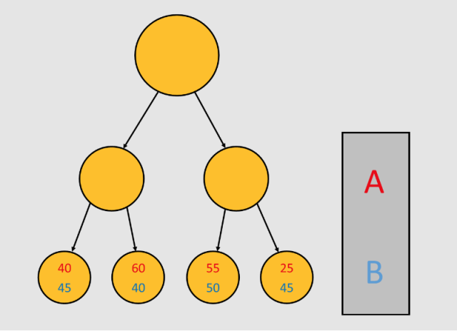
A should think carefully before choosing the left node.

A few subtleties emerge. Player A, who is to make the first move, observes that the second-to-left node in the bottom row promises a payoff of 60. Should A choose the left node in the middle row? Not so fast. If A chooses left, then B, faced with a choice between 45 and 40, will select the former, excluding the outcome paying 60 and offering A only 40. A projects similarly that if he chooses the right node, B, faced with a choice between 50 and 45, will again select the former, offering 55 to A.

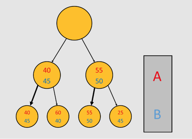
Intermediate nodes can be marked with their projected outcomes under optimal play.

The outcome of this reasoning is presented in the diagram above. A, forecasting B’s response to each of his possible immediate choices, may assign to each of these immediate choices a further pair of payoffs, essentially indicating how things would go given that choice. In effect, these new pairs are “lifted” to each node A could choose from the subsequent node that B would choose. Each such winning choice is marked with a bold arrow.

The top node ends up marked with the final outcome of optimal play.

This done, the proper choice for A is revealed simply by a choice between two utility values. A, knowing how things would go for each of his choices, simply chooses that which promises the most utility. This is described in the diagram above. The values in the topmost node, after one further “lift”, indicate the final payoff accorded to the two players at the end of optimal play.

An algorithm for perfect play in finite sequential games

This sort of reasoning can be extended to a general recursive procedure for determining optimal play in a finite sequential game. We start with a tree, in which the nodes in each successive row are assigned to a player, and this assignment is alternating; this tree is balanced in the sense that each path from root to leaf has the same length; finally, we assign to each leaf in the tree a pair of numbers corresponding to that outcome’s payoffs. How should each player play?

Each player should always choose, among the presently available nodes, that promising the highest utility to him. Of course, this promised utility must be determined by the opponent’s projected reactions to each possible choice; the first player of course knows that this opponent’s determination will itself be informed by the opponent’s projection of the first player’s reactions to each of his choices; at infinitum.

We must traverse the tree. In a bottom-up manner, given each family consisting of a node and its children, we lift the payoff pair corresponding to the child delivering the highest utility to the player active in the child’s row. In each such case, we also indicate the link between the parent and the winning child with a bold arrow. Lifting optimal play up the tree, we end up with a pair of values at the top – these indicate the final utility values conferred given optimal play – together with a trail of bold arrows tracing out the path of this play. (Note: a trail of bold arrows will extend beneath each node, and not just those involved in optimal play. This is good: if one player slips, the other can carry on along the new path.)

I’ll describe this algorithm in pseudo-pseudo-code – that is, plain English – before writing it in pseudo-code. Here’s the former:

• Procedure: Assign score to a node
  • If this node is a leaf, then it already has scores. Exit the procedure.
  • Recursively call the procedure on each of this node’s children.
  • Among this node’s children, determine that which confers the highest utility to the player opposite the player associated with the parent.
  • Copy that child’s scores to the parent node. Mark that child as the winner.
  • Exit the procedure.

The effect of calling this procedure on our tree’s root –- as anyone familiar with recursion will see –- is to traverse the tree bottom-up, lifting the proper score (and marking the winner) at each stage.

Here’s the algorithm in pseudo-code. I’ll define an object and a routine:

• object Node
  • List children
  • boolean player // 0 for A, 1 for B
  • integer array[2] scores
  • Node winner
• function score (node)
  • if (node is leaf) return
  • integer max = -∞
  • for each child of node
    • score(child)
    • if (child.scores[!node.player] > max)
      • max = child.scores[!node.player]
      • node.scores = child.scores
      • node.winner = child
  • return

This algorithm determines optimal play in finite games.

Minimax and dominant strategies

The above algorithm can be characterized in the following way:

For each of A’s choices, determine the response best for B. Among A’s choices, choose that for which the response best for B is best for A.

In the special case of a zero-sum game, like tic tac toe or chess, what’s best for A is worst for B, and vise versa. In this situation, the above rule can be rephrased from A’s point of view:

For each of A’s choices, determine the most threatening possible response. Among A’s choices, choose that for which the most threatening response is least threatening.

This is the source of the term minimax, used to describe the sorts of strategies employed in two-player games. Indeed, A’s role here is precisely to minimize, over the set of his possible choices, the maximum loss given that choice. Of course, the term embodies a simplification. The recursion is not two steps deep, but arbitrarily so. (Minimaximinimaximin___ didn’t have the same ring to it.)

Of course, in chess, it’s much less clear that games are finite — they are, provided that certain esoteric rules are enforced. Even assuming they are, the recursive algorithm described above would take longer — much, much longer — to bottom out. In practice, this exhaustive search strategy is doomed to fail; modern chess engines combine tree pruning with an evaluation function which evaluates (non-terminal) nodes on their own merit rather than through a search to the bitter end. In any case, the reasoning is similar.

We also describe the notion of dominant strategy. A certain player – say A – has a dominant strategy just when optimal play, if followed, takes him to victory. Of course, we should clarify what victory means. If, in the above example game, we declared A the victor just when he finishes with a score higher than B’s, then A has a dominant strategy. If we required for A to win that he end with a score of 60 or above, then A does not have a dominant strategy in the above game.

In practice, payoff pairs will be simple, and victory will be straightforward to define. Indeed, the most important case in practice will be that in which each payoff pair simply assigns a 1 to one player and a 0 to the other. In this case, it’s clear what victory means: Ending with a 1. In particular, there are no draws, though one game may feature many paths to victory. Here, we can rephrase our strategy once again:

For each of A’s choices, determine whether any responses lead to victory for B. Among A’s choices, choose one in which all of B’s responses lead to defeat.

A has a dominant strategy precisely when the execution of this dictum is possible.

A dominant strategy exists for one player in every finite game. This is proven essentially by construction — in fact, by the algorithm given above. The question of whether dominant strategies exist in infinite games is highly subtle. For certain infinite games — that is, for certain victory subsets of the set of countably infinite sequences of integers — it is known that winning strategies exist. (These determined victory sets include, for example, clopen sets in the Baire space, and, more generally, Borel sets [2]). In other cases, meanwhile, determinacy is a matter of axiom! This is, of course, nothing other than the Axiom of Determinacy.

Frankly, it’s difficult for me to grasp how exactly it could be the case that no dominant strategy exists for either player (in an infinite game, of course). I will leave this for future thought, mine and yours.

Two-player games and mathematical proofs

This sort of situation naturally occurs in math. Many mathematical proofs feature so-called bounded quantification — in which objects are quantified over some restricted set — and, in particular, the alternation of universal (i.e., for all) and existential (i.e., there exists) bounded quantifiers.

The sequential game is just the structure we need to capture alternating bounded quantifiers. To suggest this point by example, we can rephrase the victory condition once more. A has a dominant strategy exactly when the following is true:

There exists a choice available to A for which for all of B’s subsequent responses, B loses.

The truth of this statement — involving alternating quantifiers — coincides with the existence of a dominant strategy for its associated game. I’ll describe, more generally, a process by which we can associate, to each statement featuring alternating quantifiers, a two-player game, the existence of a dominant strategy for a certain player of which coincides with the truth of the statement.

Take for example a sentence involving quantification, like: There exists an x in the set X such that for all y in the set Y_x (which possibly depends on x), the function f(x, y) = true. We can construct a two-player game as follows. We let A be the first player, and we let the first row of options available to him be the members of the set X. For each choice x, we let the collection of B’s responses to x be the members of the set Y_x. Finally, to each y in each Y_x we associate a payoff pair which gives to A f(x, y) and to B !f(x, y). P is true just when A has a dominant strategy.

This construction generalizes easily to quantified statements of arbitrary length. Each set over which quantification occurs stands for a node of the tree (the first set is the root). Each member of this set stands for a child of this node. Finally, each move in the game selects one of these children and initiates quantification over the set it represents. Let A play whenever there exists occurs; let B play whenever for all occurs. Once again, P is true exactly when A has a dominant strategy. (A might not be the first player.)

The connection between alternating quantification and sequential games is uncanny. The successive restriction of the set over which quantification occurs is exactly captured by the way in which successive choices restrict the size of the tree over which play occurs. The alternation of for all and there exists corresponds, in short, to minimax. The adversarial nature of two-player games is such that victory is possible precisely when a certain alternating quantification holds true.

It’s well known that the negation of a statement containing alternating quantifiers is equivalent to the statement in which all quantifiers have been “flipped” (i.e., ∀ becomes ∃ and vise versa) and the innermost statement has been negated. (For example, ¬(∃ x ∈ X s.t. ∀ y ∈ Y_x, f(x, y)) ⇔ ∀ x, ∃ y ∈ Y_x s.t. ¬f(x, y).) This, too, has an interpretation in the language of sequential games. Translating both sides of an equivalence of the above sort into the language of game theory, we produce the statement that A fails to have a dominant strategy in some game just when A does have a dominant strategy in the same game, provided that the two players reverse their roles and all payoffs are flipped. This, of course, is the same as saying that B has a dominant strategy in the original game. We’ve recovered the transparent fact that B has a dominant strategy just when A does not.

A familiar example comes from the usual characterization of openness (in the standard topology) for subsets of Rⁿ. (Whether this is a definition or a consequence depends on our definitions.) A subset U of Rⁿ is open iff for each point x in U, there exists an open n-ball D containing x such that D is contained in U. This is equivalent to the existence of a dominant strategy for A in the following game:

B: Choose a point x ∈ U.
A: Respond with an open ball D ∋ x.
If D ⊂ U, A gets 1 and B gets 0. Otherwise, A gets 0 and B gets 1.

Each subset of Rⁿ has a certain two-player game attached to it; to prove that some given set U is open, one must demonstrate the existence of a dominant strategy for A in U‘s corresponding game.

This, in fact, is just one example in a broad class of so-called topological games, two player games involving choices of objects in a topological space. We just saw that openness of a set can be characterized by the existence of a dominant strategy in a certain topological game associated with the set. In fact, many deep properties of sets in topological spaces have characterizations in terms of topological games. In the Banach–Mazur game attached to a fixed subset A of a topological space X, players take turns extending a chain B₁ ⊃ A₁ ⊃ B₂ ⊃ A₂ ⊃ … of successively smaller open subsets of X, with the proviso that the second player, A, wins just when the infinite intersection of the sets A_n with A is nonempty. It’s known that this second player has a dominant strategy precisely when A is residual in X, that is, its complement is meagre [3].

As fascinating as this is, I’ll now move onto other things.

Minimax beyond sequential games

Minimax reasoning in chess has fascinating manifestations among its experts. Chess players regularly explore variations running as many as ten or twelve moves deep. In doing so, these players — perhaps unwittingly — perform many-layered minimax calculations on the fly.

The presence of this sort of reasoning is detectable in the way these players describe their thought processes. “This attack is good because the apparent counter-threat posed by the pawn isn’t real,” a player might say. “If the pawn recaptures, it opens up a file revealing an attack on the queen.” This simple statement, its sort familiar to chess players, disguises a minimax argument running three layers deep. Even more simply: “This variation isn’t worth pursuing. He would never move his piece there. I’d just take it.” The phrase I just take it, ubiquitous among chess players, itself reveals a minimax idea: It describes a move by, say, A, for which the best response for B does not lead to the best outcome for A. In chess, one plays with the understanding that his opponent will respond with the best possible move, a move whose quality is determined by its possible continuations, and so on…

This general philosophy of minimax, I contend, extends yet further to games which are not strictly sequential and which perhaps aren’t games at all. Imagine, for instance, the case of a boxing match. Though boxing is not strictly sequential in the way that chess is, it has a sequential character, with the feature that future positions (which deliver different values to the players) are affected to at least some degree by immediate moves. If a boxer “plays” the “move” “drop both hands”, the opponent can respond with “right hook to the jaw”; if he instead plays “dodge left”, the opponent’s available responses might lead to more favorable continuations. Soccer, say, also shares these features, as do many other sports.

Even philosophy, I argue, features minimax characteristics, where games, here, are played by a philosopher against his rivals, or, if you like, against truth itself. Each argument employed by the philosopher must face an array of possible counter-arguments. Some of these arguments, near-tautologies, will inspire few counter-arguments yet wind up too weak to demonstrate anything contentious; others, overly ambitious, would yield success did they not fall to deft counter-arguments. The arguments which succeed are, again, those that assert just enough nuance to overcome all possible continuations, and which yet still achieve the desired result. The structure of philosophical arguments is, of course, highly complex (probably analogous in many ways to that of mathematical arguments, which has been described thoroughly in this series). This logical complexity, though, only further opens the door to minimax reasoning.

An example is visible in a comment written on this blog by a philosopher and friend, Richard Teague. Richard describes the obstacles faced by an argument put forth by Wittgenstein:

If we accept this point from Witt. then we must accept that if one thinks that P, then one must be able to be certain, upon reflection, that one is thinking that P. But, as you can see, this recurses to generate a sort of ‘omega-sequence thought’ of the form ‘I am certain that I am certain that I am certain that … I am certain that I am thinking that P’. But we cannot think this thought, can we? … If not, then the requirement of the capacity for certainty means that we’re never certain that we’re thinking any particular thought… Indeed, Witt.’s conclusion is that we do not think in this way.

Though the reasoning is complicated, at least three levels of minimax are present.

I argue finally, that minimax is very much present in mathematics itself, even in proofs which do not (explicitly) involve alternating quantifiers. In essence, the argument for this presence is the same as that given for philosophy. The game, of course, is played against truth itself. The successful proofs are those which overcome an elaborate minimax game. In each of the many steps of a successful proof, the mathematician plays a move which is just ambitious enough to generate progress, but which is not such as to generate insurmountable difficulties. Tracing his way through an elaborate tree, he lands on the desired node.

Thus, we have a final characterization of mathematical proof: A proof is a demonstration that a certain two-player game has a dominant strategy.

Perhaps Fields Medalist Charles Fefferman put it best when he said:

Math is like playing chess but you are playing a game against the devil. But you get to take steps back; you get to take back as many moves as you like. So if you play against the devil, you get crushed and you think about why you lost and you try to change your move and again you are crushed; you are simply wrong, whatever reason you thought was the reason for you being crushed that’s not the reason at all. But sooner or later maybe you get an idea and then you get a little scared to play and get crushed again, but you give it a try because the devil will have to make another move, and pretty soon after a few years of playing many games, you start to see what is going on, and after a while of fighting, you win. But while you play this game God is whispering in your ear “move your pawn over there, is all you have to do and then he is in real trouble.” But you can’t hear, you are deaf… well not deaf, but you have to pay a lot of attention because if not, you can’t know what God is telling you. But that is the spirit of the thing. (Interview in [4], corrections due to [5])

References:

1. Bourbaki: Foundations of Mathematics for the Working Mathematician
2. Wikipedia: Axiom of Determinacy
3. Cao, Moors. A Survey on Topological Games and Their Applications in Analysis
4. ciencianostra: “Math is a chess game against the devil”
5. Gypsy Scholar: The Tao of Mathematics: Playing Chess with the Devil